TSTN-058

AOS Control Loop Testing with Open-Loop Reproductions

This is a draft.

By:

• Craig S. Lage

Abstract

The MTAOS control loop is complex and has many parameters. In addition, because the measured Zernikes are noisy, and because of night-to-night variation, it is difficult to make definitive tests on sky. This technote describes a simulation package that allows testing alternate control loop schemes using on-sky data from which the calculated corrections have been removed, giving an effective stream of open-loop Zernike measurements. First results from the simulator are presented, including comparisons of different correction strategies, an investigation of Degree-of-Freedom (DoF) versus virtual-mode (Vmode) control, a study of the Z4/Z11 cross-coupling, control in Zernike input space, and the addition of an optional Kalman filter.

Acknowledgements: Aaron Roodman, Guillem Megias, Tiago Ribeiro, and Chuck Claver.

Introduction

The MTAOS active optics system corrects wavefront errors in the Vera C. Rubin Observatory by adjusting the Camera and M2 hexapods and the M1M3 and M2 mirror bending modes. Corrections are calculated from Zernike coefficient measurements at four corner detectors and are applied once per visit. Testing different control strategies on sky is difficult because (a) Zernike measurements are noisy, (b) sky conditions vary from night to night, and (c) each on-sky test consumes precious observing time.

This technote describes a software simulator that sidesteps these difficulties by replaying a recorded night of data in simulation. The key idea is the open-loop reproduction (OLR): the accumulated degree-of-freedom (DoF) corrections (the trim) are subtracted from the measured Zernikes, reconstructing what the wavefront would have looked like had no corrections ever been applied. Any PID control strategy can then be applied to this OLR stream, allowing a direct, reproducible comparison of different strategies against real atmospheric and instrumental disturbances.

Terminology used throughout this document follows the conventions of Aaron Roodman:

• Tweak — the per-visit change in DoFs commanded to bring the Zernikes to their target values (called visit_dof in the EFD).

• Trim — the accumulated sum of tweaks (also called dof_state). The trim does not include the Look-Up Table (LUT) correction.

The simulation code is available at: https://github.com/lsst-so/ts_aos_analysis/blob/tickets/RSO-441/notebooks/pid_simulations/PID_Loop_Simulation_Kalman_04May26.ipynb

Methodology

The simulation proceeds in three steps.

Step 1 — Build the open-loop reproduction. For each exposure in a chosen night, the recorded Zernike deviations and the applied trim (dof_state) are read from the nightly parquet file. The sensitivity matrix \(S\) (mapping DoF changes to Zernike changes) is used to add back the effect of the trim, yielding the open-loop Zernike stream:

\[\mathbf{z}_\mathrm{OLR}(N) = \mathbf{z}_\mathrm{meas}(N) + S\,\mathbf{t}(N)\]

where \(\mathbf{t}(N)\) is the trim applied before exposure \(N\).

Step 2 — Run the simulated PID loop. Starting from zero trim, the OLR Zernikes are fed through the PID controller visit by visit. At each step, the current trim is subtracted from the OLR Zernikes (via applyTrim) to obtain the simulated Zernikes, which are passed to getTweak (the OFC) to compute the next correction. The correction is accumulated into the trim and the loop advances to the next visit.

Step 3 — Analyse and plot results. Simulated Zernike residuals, DoF/Vmode trims, integral terms, and the AOS contribution to the PSF FWHM are available as stored arrays and can be visualised with the built-in plotting methods.

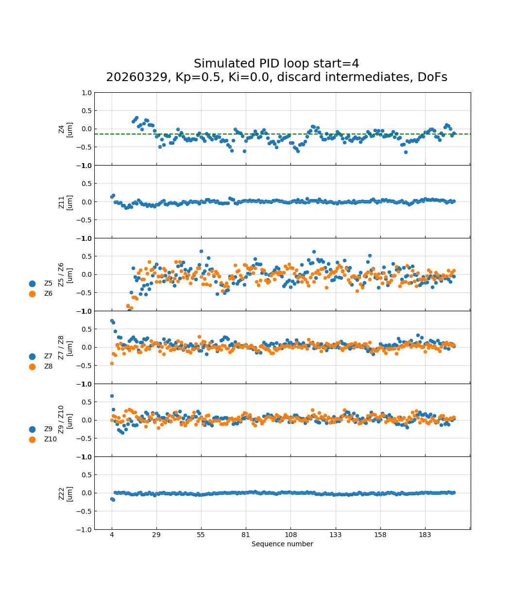
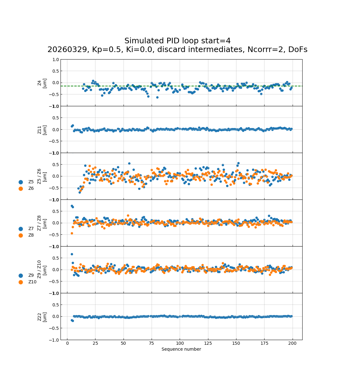
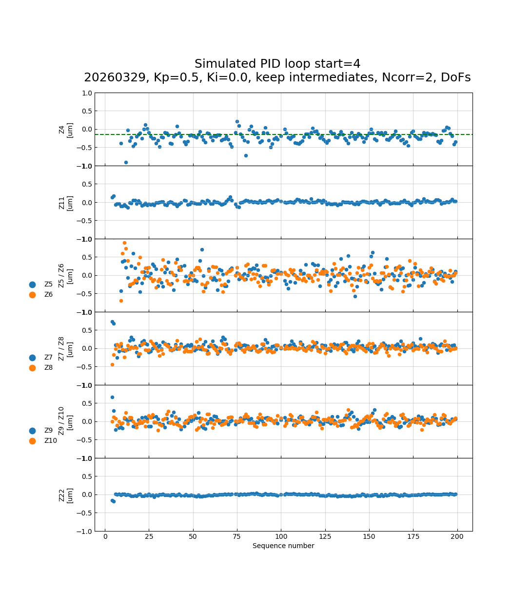
Two correction lag modes are supported, illustrated in Fig. 1 and Fig. 2:

• discard_intermediates=True — a new tweak is computed only every \(N_\mathrm{corr}\) visits; intermediate visits use the last applied trim unchanged.

• discard_intermediates=False — a new tweak is computed every visit but applied with a lag of \(N_\mathrm{corr}\) visits, mimicking the pipeline processing delay.

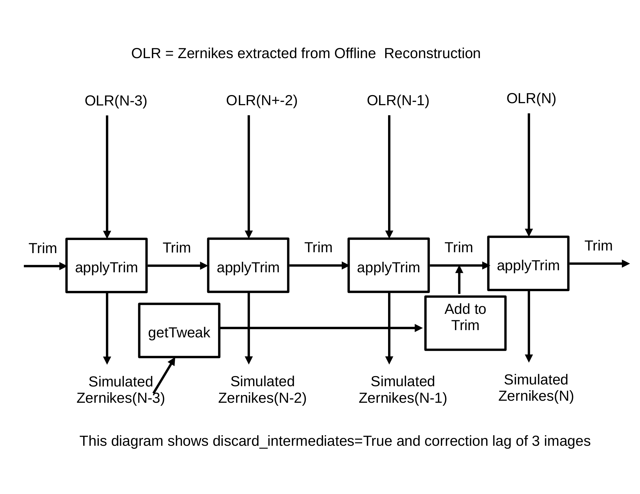
Fig. 1 Schematic of the discard_intermediates=True strategy with a correction lag of three visits. A tweak is calculated from the simulated Zernikes at exposure \(N-3\) and added to the trim before exposure \(N\). Intermediate exposures use the unchanged trim.

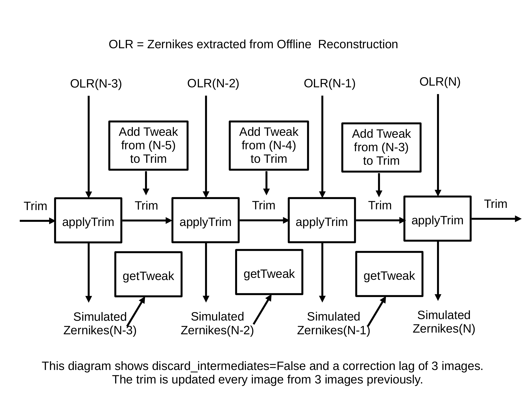
Fig. 2 Schematic of the discard_intermediates=False strategy with a correction lag of three visits. A new tweak is computed every visit but the tweak applied to visit \(N\) was computed three visits earlier, so every visit benefits from the most recent available correction.

Open-Loop Reconstruction

Fig. 3 shows the OLR Zernike stream (circles) alongside the original measured Zernikes (crosses) for the night of 20260329. The OLR Z4 signal is notably larger than the measured value because the Camera and M2 dZ trims — which had been suppressing the Z4 error — have been removed. The OLR stream is the “true” open-loop disturbance that the PID loop must learn to reject.

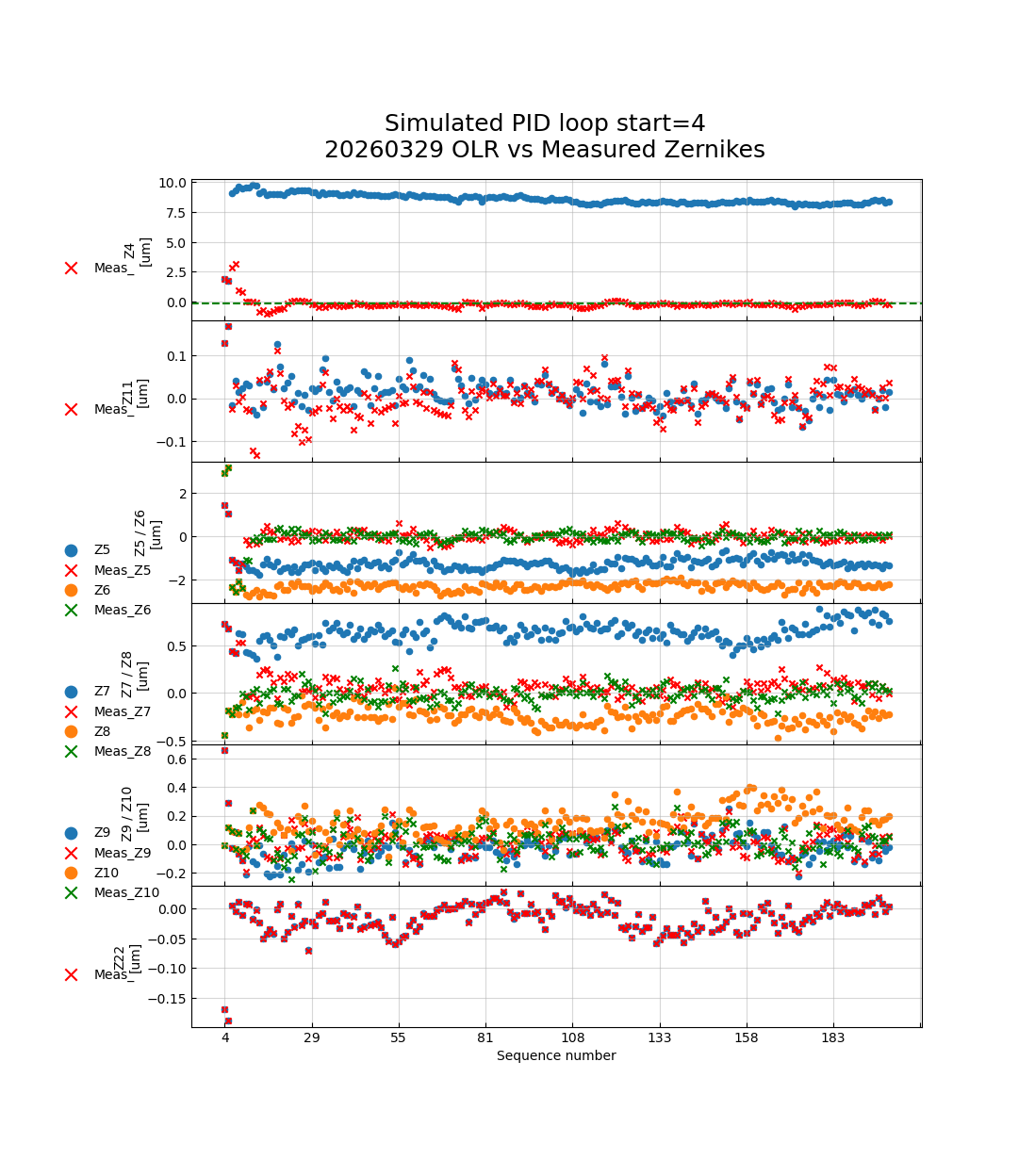
Fig. 3 Open-loop reproduction (circles) versus measured Zernikes (crosses) for night 20260329. The large OLR Z4 signal reflects the dZ trims that have been removed.

Impact of Intermediate Updates

Correction Lag of N+3

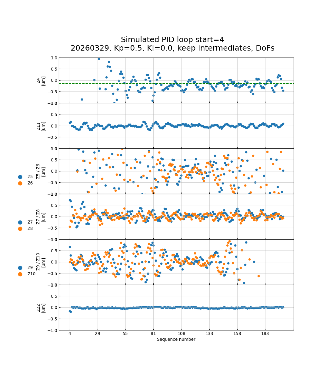
Fig. 4 through Fig. 7 compare Kp = 0.3 and Kp = 0.5 with and without discarding intermediate updates, using a correction lag of three visits.

With discard_intermediates=True the loop is stable for both gain values. With discard_intermediates=False and Kp = 0.5, the loop begins to oscillate — a well-known consequence of the three-visit lag acting with high gain. Even with Kp = 0.3 oscillations are beginning.

Fig. 4 Kp=0.3, discard intermediates, N+3	Fig. 5 Kp=0.3, keep intermediates, N+3
Fig. 6 Kp=0.5, discard intermediates, N+3	Fig. 7 Kp=0.5, keep intermediates, N+3

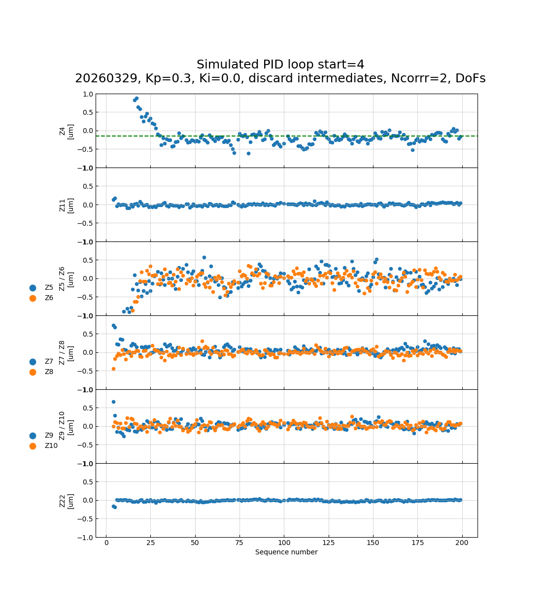
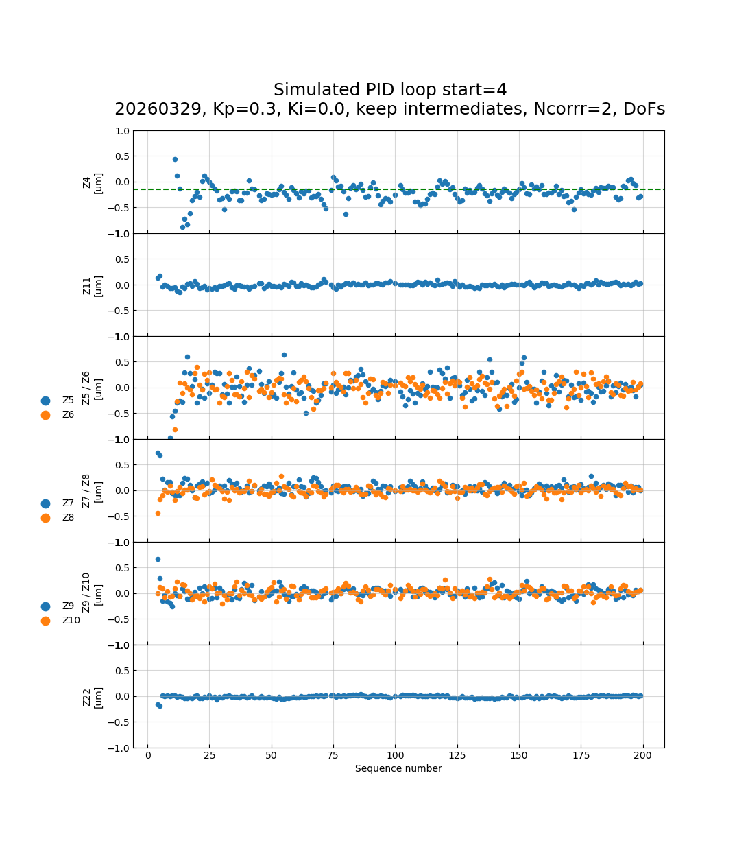
Correction Lag of N+2

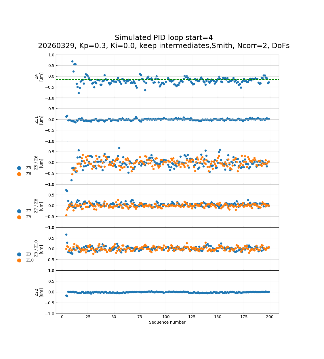
Fig. 8 through Fig. 11 repeat the comparison with a two-visit lag. Reducing the lag to two visits allows the keep-intermediates loop to remain stable at Kp = 0.5, illustrating the expected trade-off between lag and maximum stable gain.

Fig. 8 Kp=0.3, discard intermediates, N+2	Fig. 9 Kp=0.3, keep intermediates, N+2
Fig. 10 Kp=0.5, discard intermediates, N+2	Fig. 11 Kp=0.5, keep intermediates. N+2

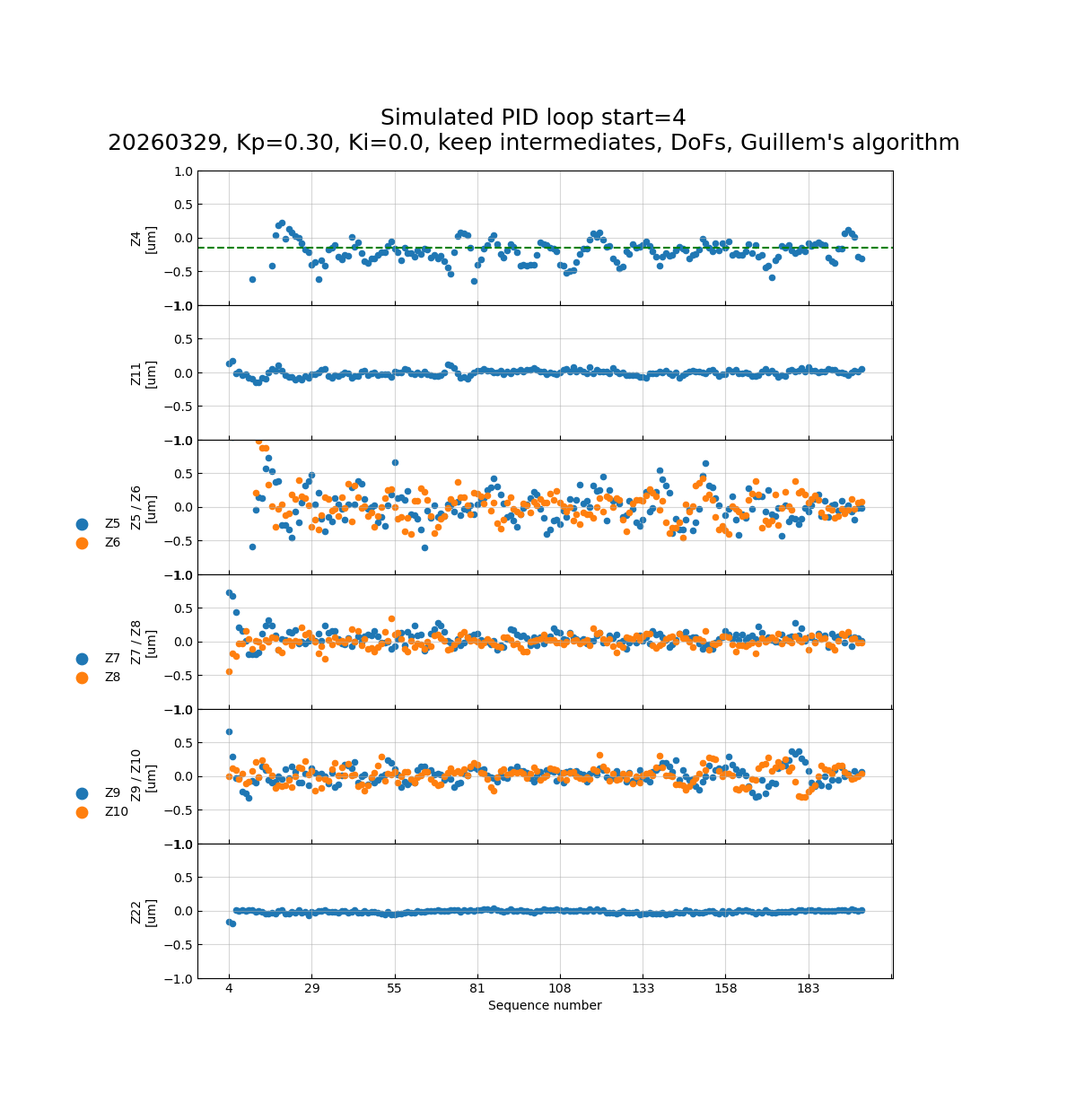
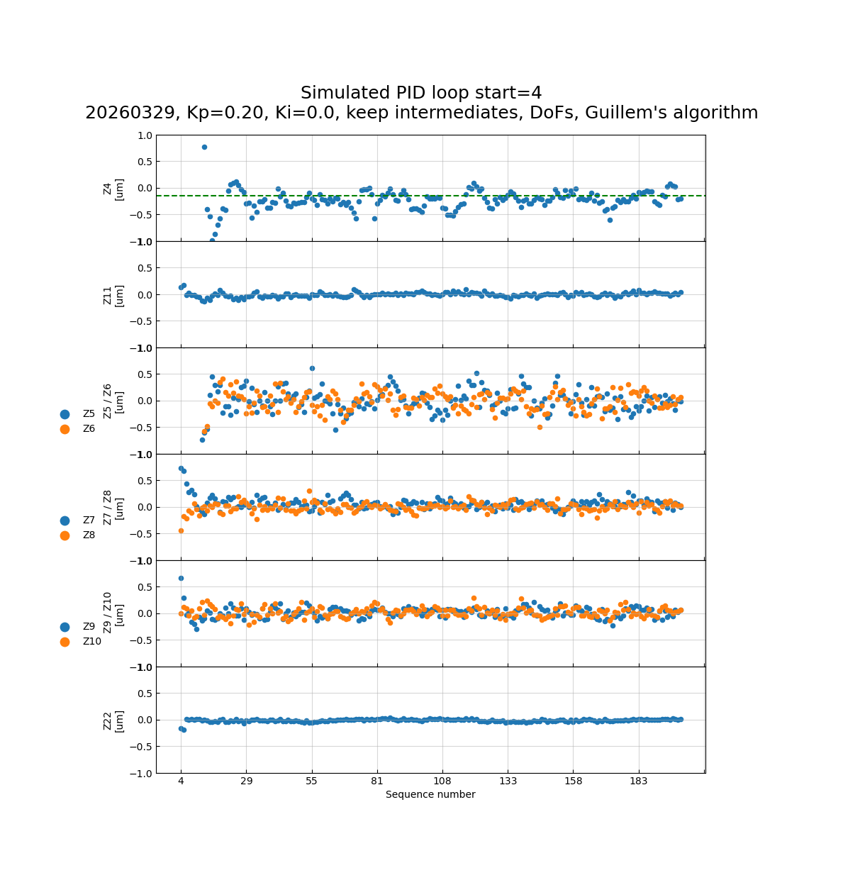
Using the Smith Predictor/Corrector

Per a suggestion from Guillem Megias, a Smith predictor/corrector can be added to compensate for the correction lag. The algorithm modifies the Zernike input to getTweak as follows:

\[\mathbf{z}_\mathrm{input}(N) = \mathbf{z}_\mathrm{sim}(N) + S\,\bigl[\mathbf{t}(N-1) - \mathbf{t}(N-2)\bigr]\]

This uses the most recent change in the trim to predict the Zernike improvement that the pending correction will deliver, effectively removing the lag from the controller’s perspective.

Fig. 12 and Fig. 13 show the improvement from the Smith corrector at N+3 lag; Fig. 14 shows the same at N+2 lag. The Smith corrector substantially reduces the residual Zernike scatter in the keep-intermediates regime with a lag of three visits, but the benefit is less clear with a lag of two visits.

Fig. 12 Kp=0.3, keep intermediates, N+3, Smith.	Fig. 13 Kp=0.2, keep intermediates, N+3, Smith.
Fig. 14 Kp=0.3, keep intermediates, N+2, Smith

How Well Do We Recover the Original Measured Zernikes?

A useful sanity check is to compare the simulated Zernike residuals with the original on-sky measurements. If the simulation is correct, running the loop with the same parameters that were used on sky should approximately reproduce the measured Zernike stream.

Fig. 15 and Fig. 16 show nights where the recovery is good. Fig. 17 and Fig. 18 show nights where significant discrepancies appear, particularly in the higher-order Zernikes. A possible explanation is that the bending-mode actuator limits applied on sky are not captured in the simulation. This needs to be better understood.

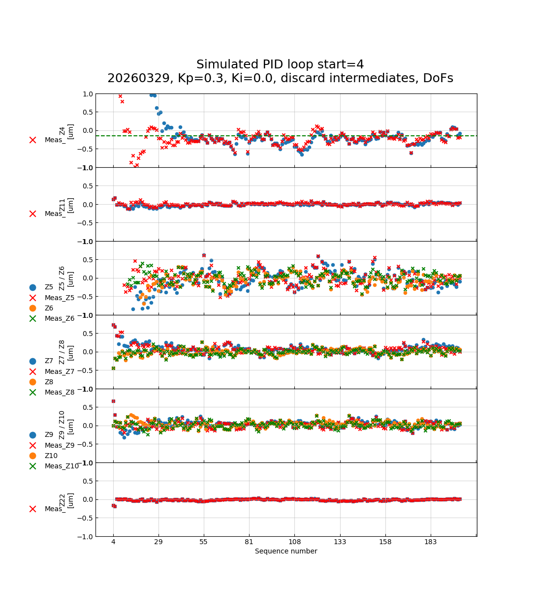
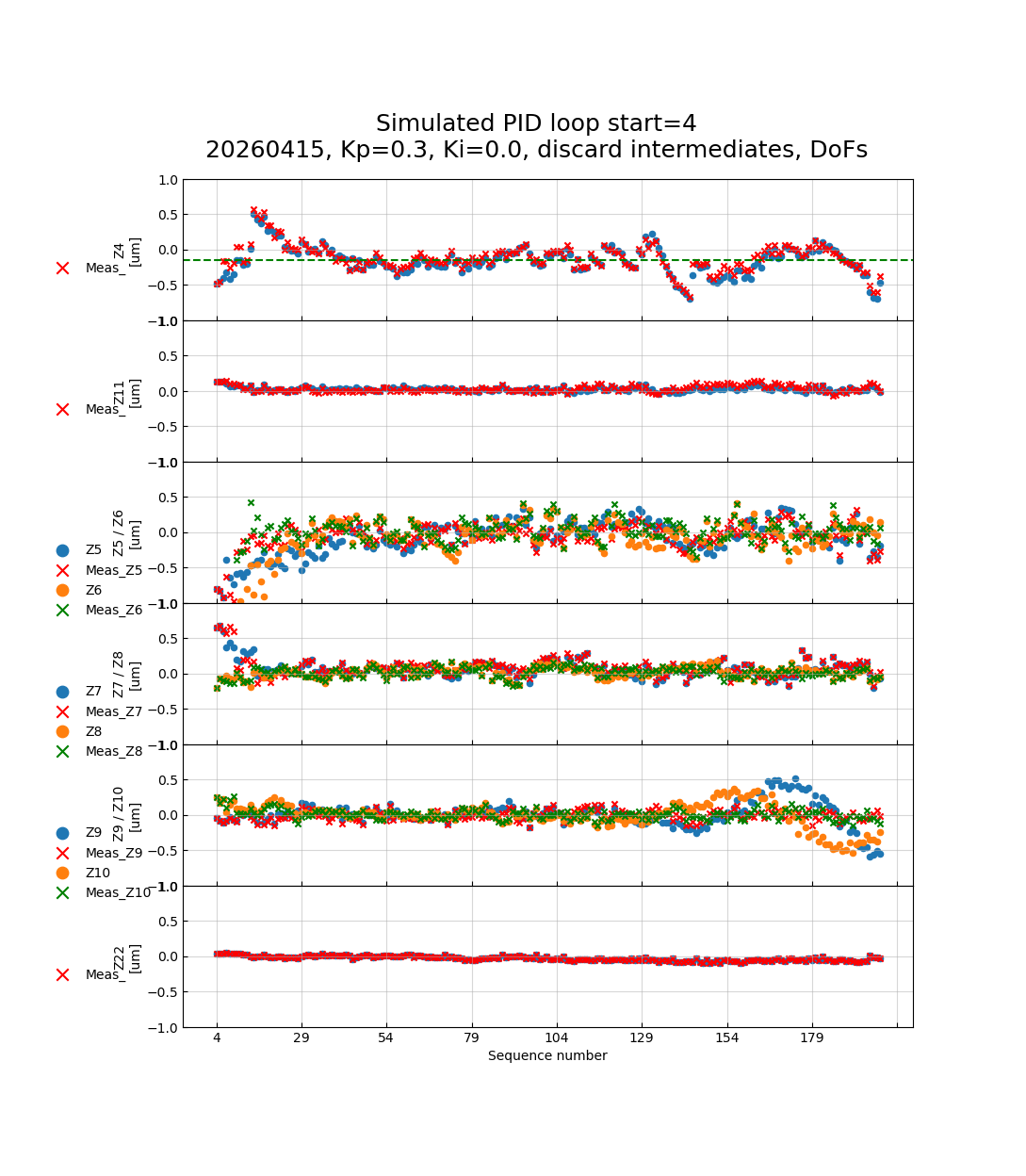
Fig. 15 Night 20260329 — simulation (circles) versus measured (crosses). Recovery is good.	Fig. 16 Night 20260415 — simulation (circles) versus measured (crosses). Recovery is good.
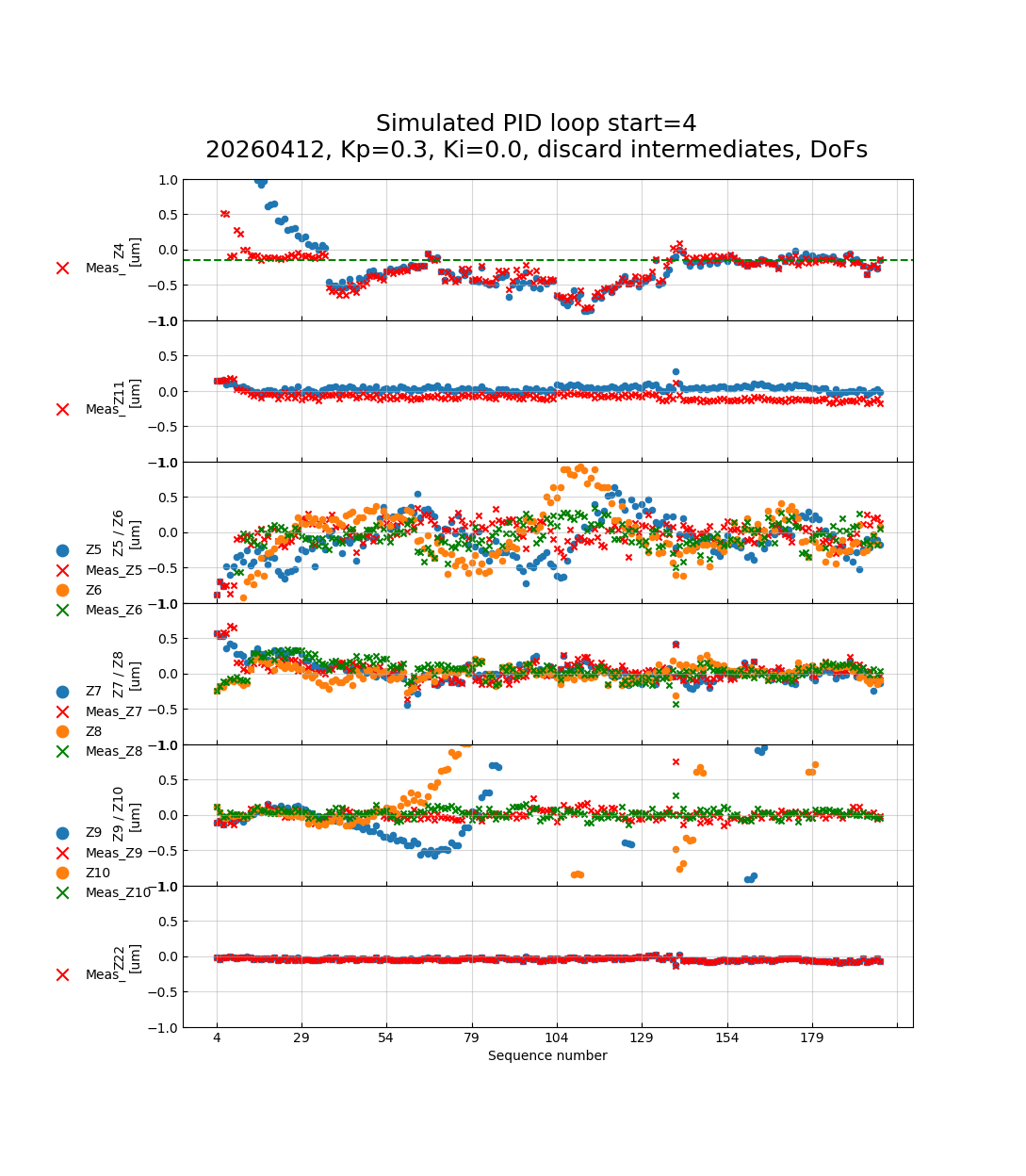
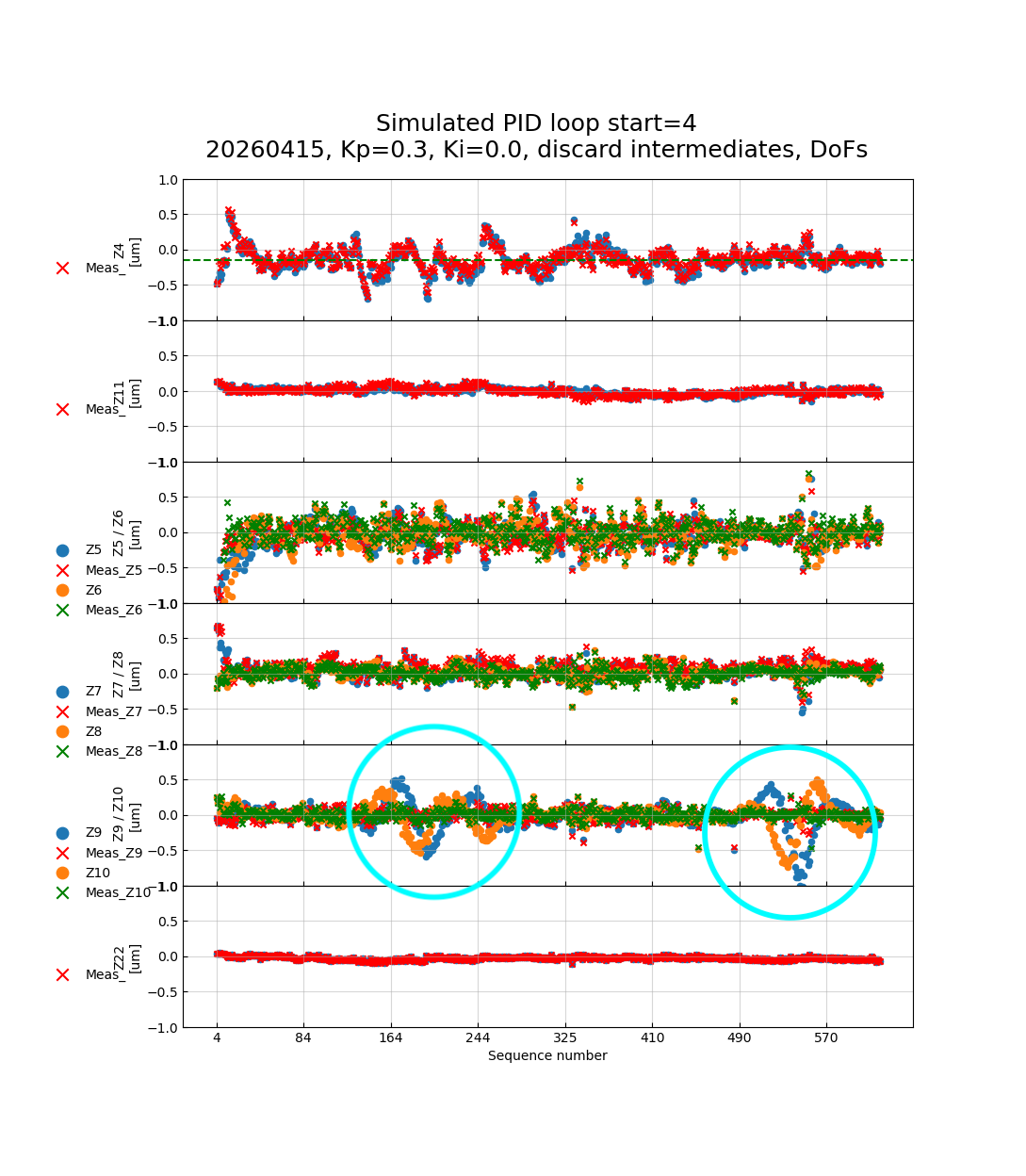
Fig. 17 Night 20260412 — higher-order Zernikes show significant disagreement.	Fig. 18 Night 20260415 (different sequence range) disagreement visible in higher-order Zernikes (cyan circle).

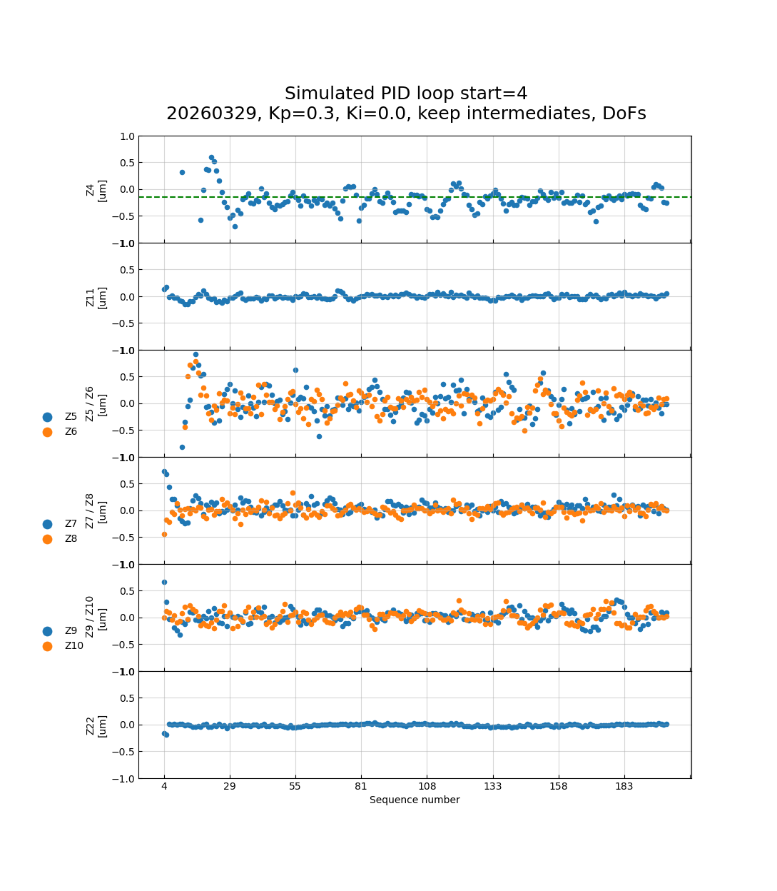
DoFs vs. Vmode Control

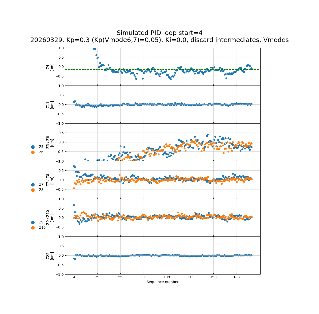
The OFC can operate in either the native DoF basis or the virtual-mode (Vmode) basis, which diagonalises the sensitivity matrix and decouples the Zernike modes from one another. Fig. 19 and Fig. 20 show that the Zernike residuals are visually identical between the two bases for the same gain values. Inspecting the stored trim arrays during the simulation confirms that the Vmodes are what is being controlled in both cases, because the OFC internally projects the DoF corrections onto the Vmode basis.

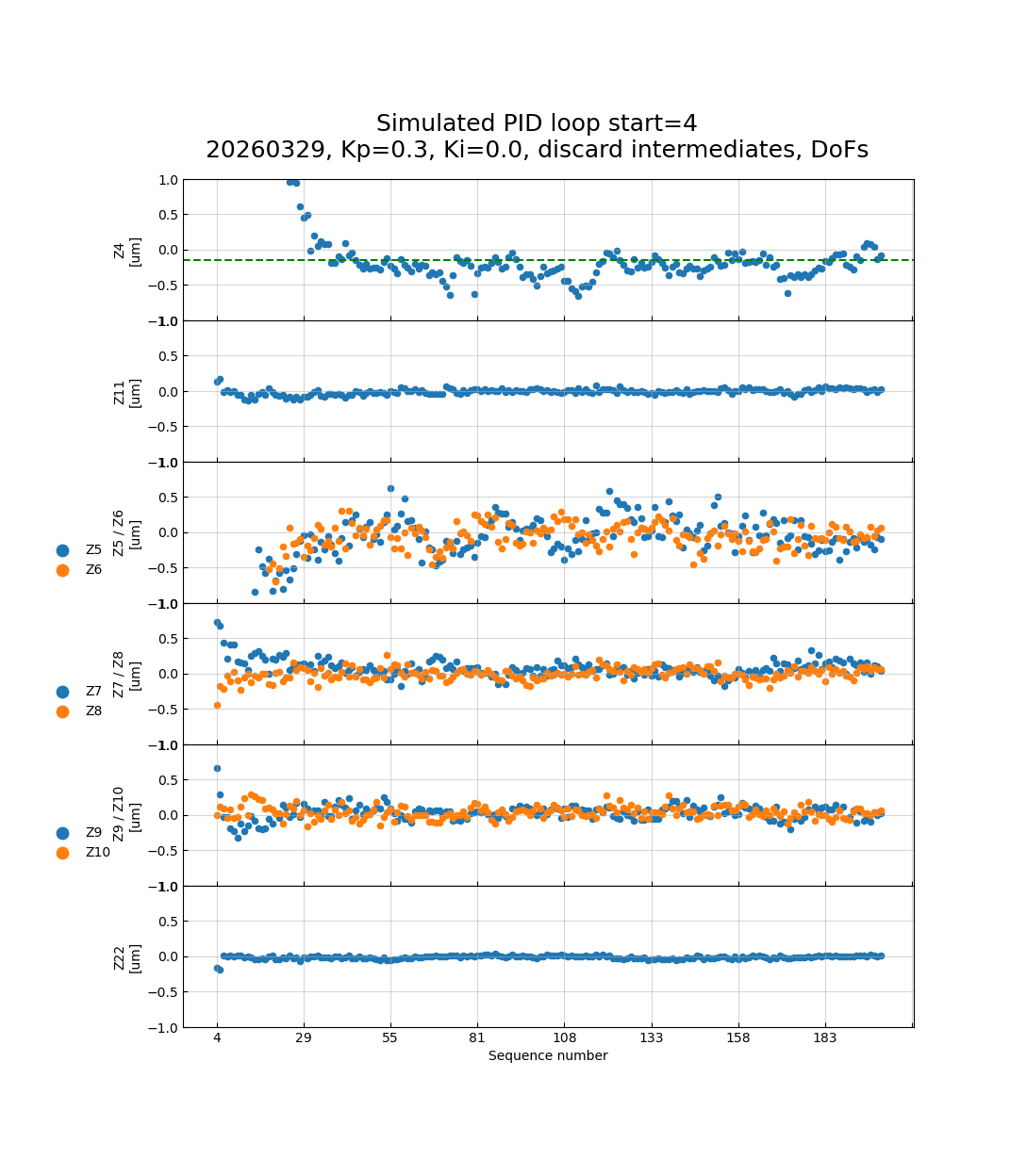
Fig. 19 DoF control, Kp=0.3, discard intermediates.

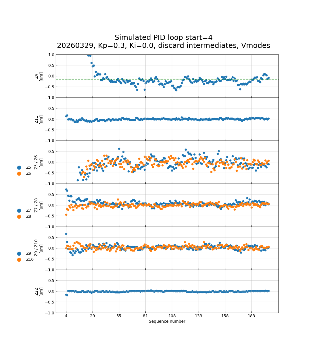
Fig. 20 Vmode control, Kp=0.3, discard intermediates. Results are visually identical to the DoF case.

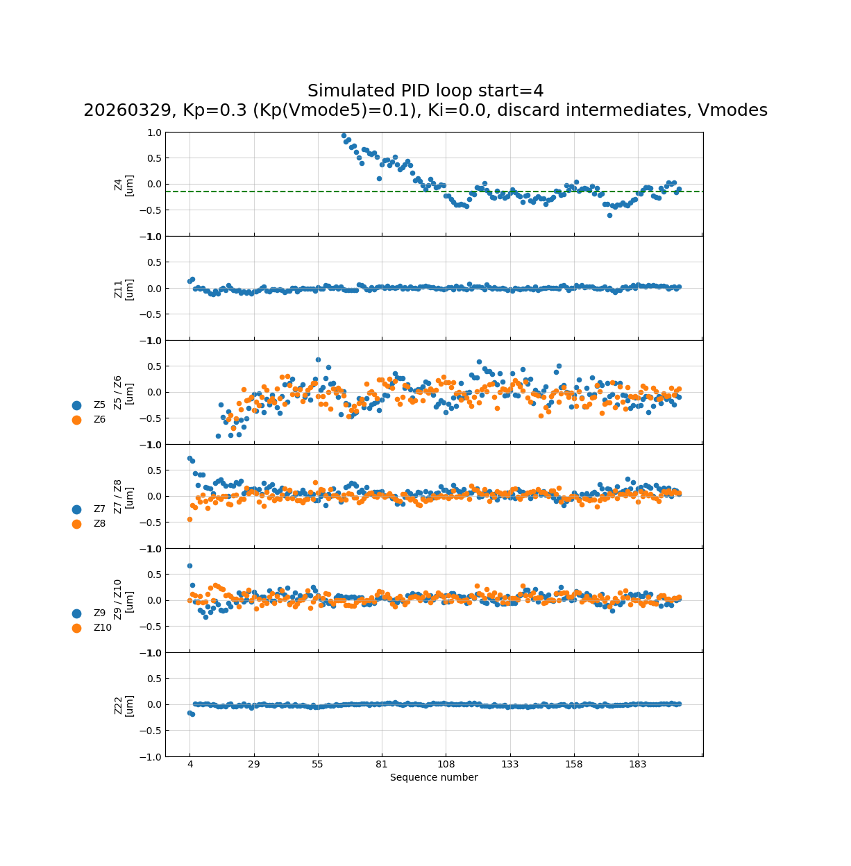
The ability to specify independent gains per Vmode was verified empirically: reducing Kp(Vmode5) from 0.3 to 0.1 visibly increases the Z4 residuals (Fig. 21), and reducing Kp(Vmode6,7) to 0.05 increases the astigmatism residuals (Fig. 22), confirming that the Vmodes are the effective control variables.

Fig. 21 Vmode control, Kp(Vmode5) = 0.1. Z4 residuals increase, as expected.

Fig. 22 Vmode control, Kp(Vmode6,7) = 0.05. Astigmatism residuals increase.

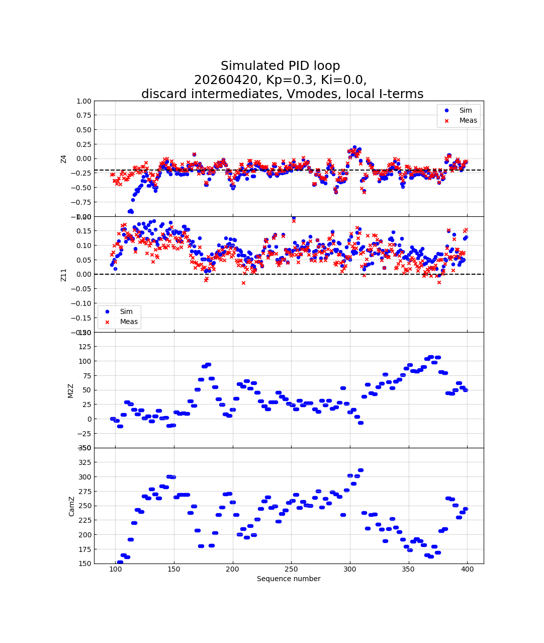
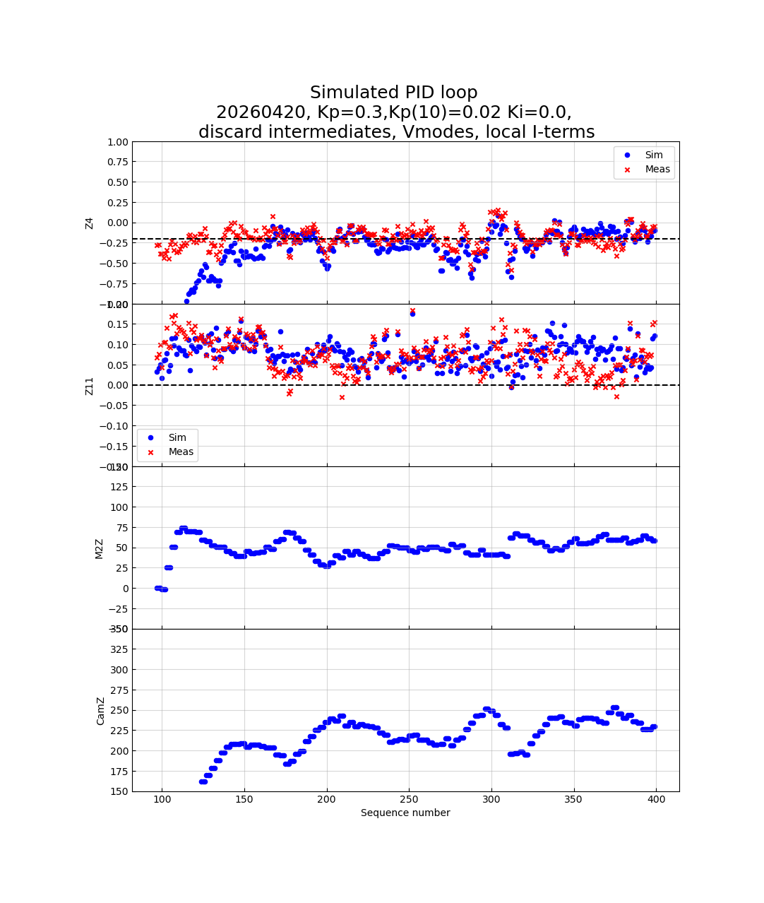
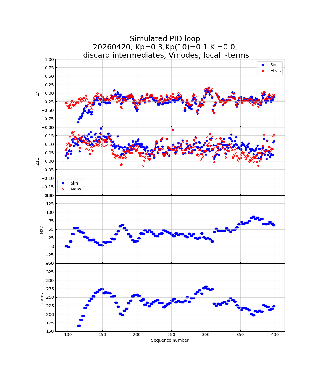
Z4/Z11 Study

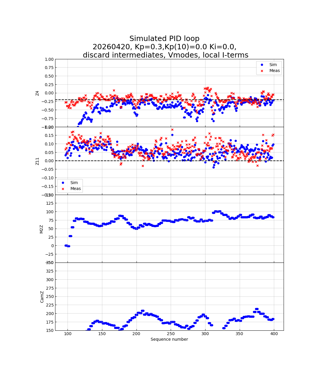
The Z4 (focus) and Z11 (spherical aberration) modes are of particular interest because they are coupled through the CamZ and M2Z actuators and tend to oscillate together. A series of simulations was run on night 20260420 to understand how the proportional and integral gains affect this coupling.

Proportional Gain Study

Fig. 23 through Fig. 26 show the effect of reducing the gain on Vmode 10 (which most strongly drives Z11). Zeroing Kp(Vmode10) removes the Z11 correction entirely, while reducing it to 0.02 provides a compromise between Z11 suppression and M2Z/CamZ stability. In both cases the opposing oscillations of M2Z and CamZ are reduced.

Fig. 23 All Kp=0.3 (baseline).	Fig. 24 Kp(Vmode10) = 0.02.
Fig. 25 Kp(Vmode10) = 0.1.	Fig. 26 Kp(Vmode10) = 0.0 (Z11 gain zeroed).

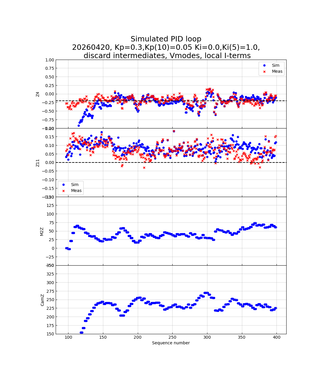
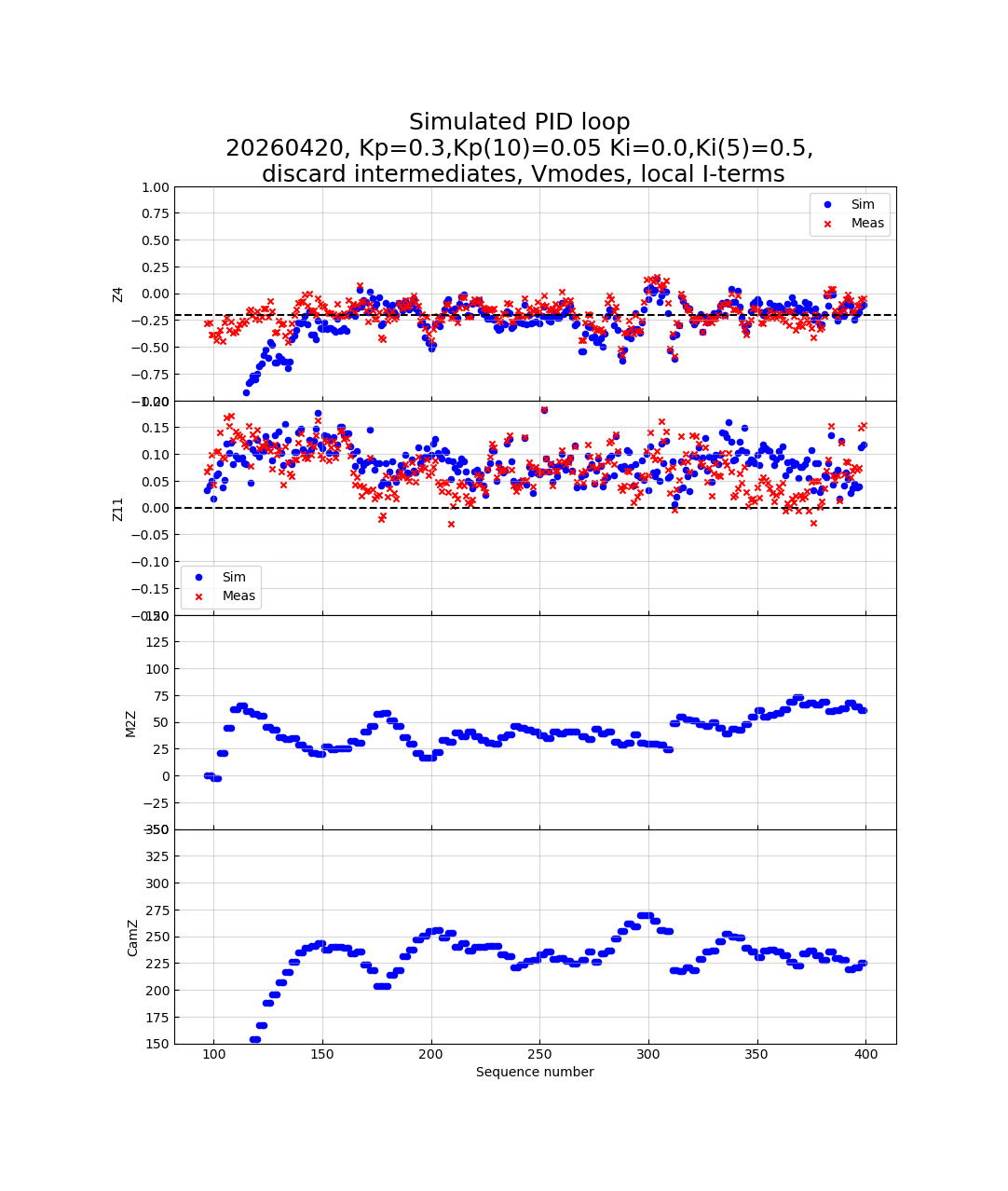
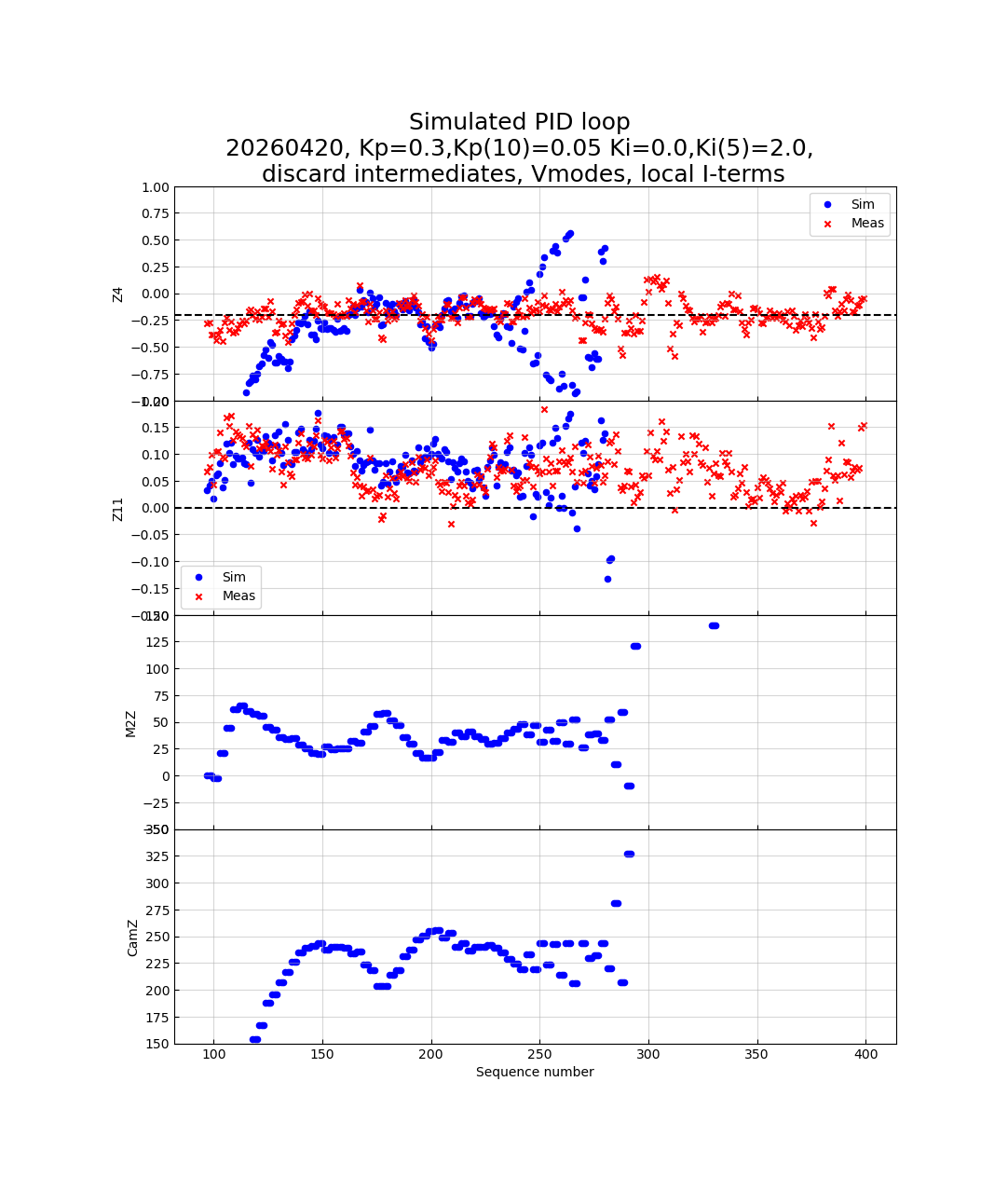
Integral Gain Study (Vmodes)

Fig. 27 through Fig. 30 explore the effect of adding an integral term to Vmode 5 (focus) while keeping Kp(Vmode10) reduced to 0.05. Adding an integral term on Vmode 5 reduces the low-frequency Z4 drift but can destabilise the loop if Ki is set too large. In general, the added control from introducing Ki is somewhat disappointing.

Fig. 27 Ki(Vmode5) = 0.2.	Fig. 28 Ki(Vmode5) = 1.0.
Fig. 29 Ki(Vmode5) = 0.5.	Fig. 30 Ki(Vmode5) = 2.0.

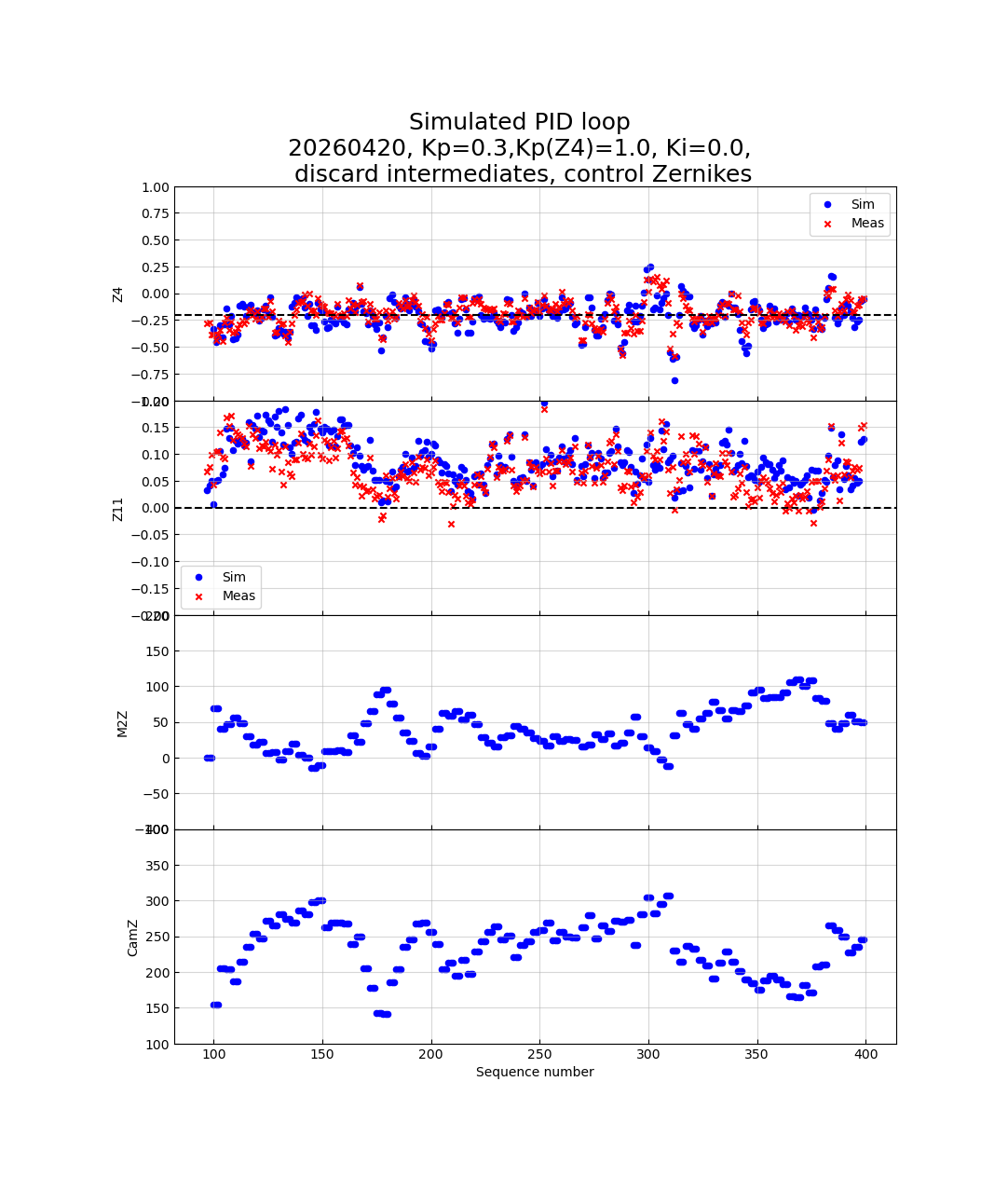
Control in Zernike Space

An option suggested by Chuck Claver is to move the PID control from the DoF/Vmode output space into the Zernike input space. In this mode the proportional and integral gains are applied directly to the Zernike measurements before they are passed to the OFC, allowing independent per-Zernike (and even per-detector) gain tuning.

Positives:

• Kp and Ki can be set independently for each Zernike coefficient and each corner detector.

• The control action is more directly interpretable in terms of the observable wavefront error.

Open questions at the time of writing:

• The Kp(Z4) gain must be set substantially higher than in DoF/Vmode control to achieve the same Z4 suppression, suggesting a scaling difference that needs investigation.

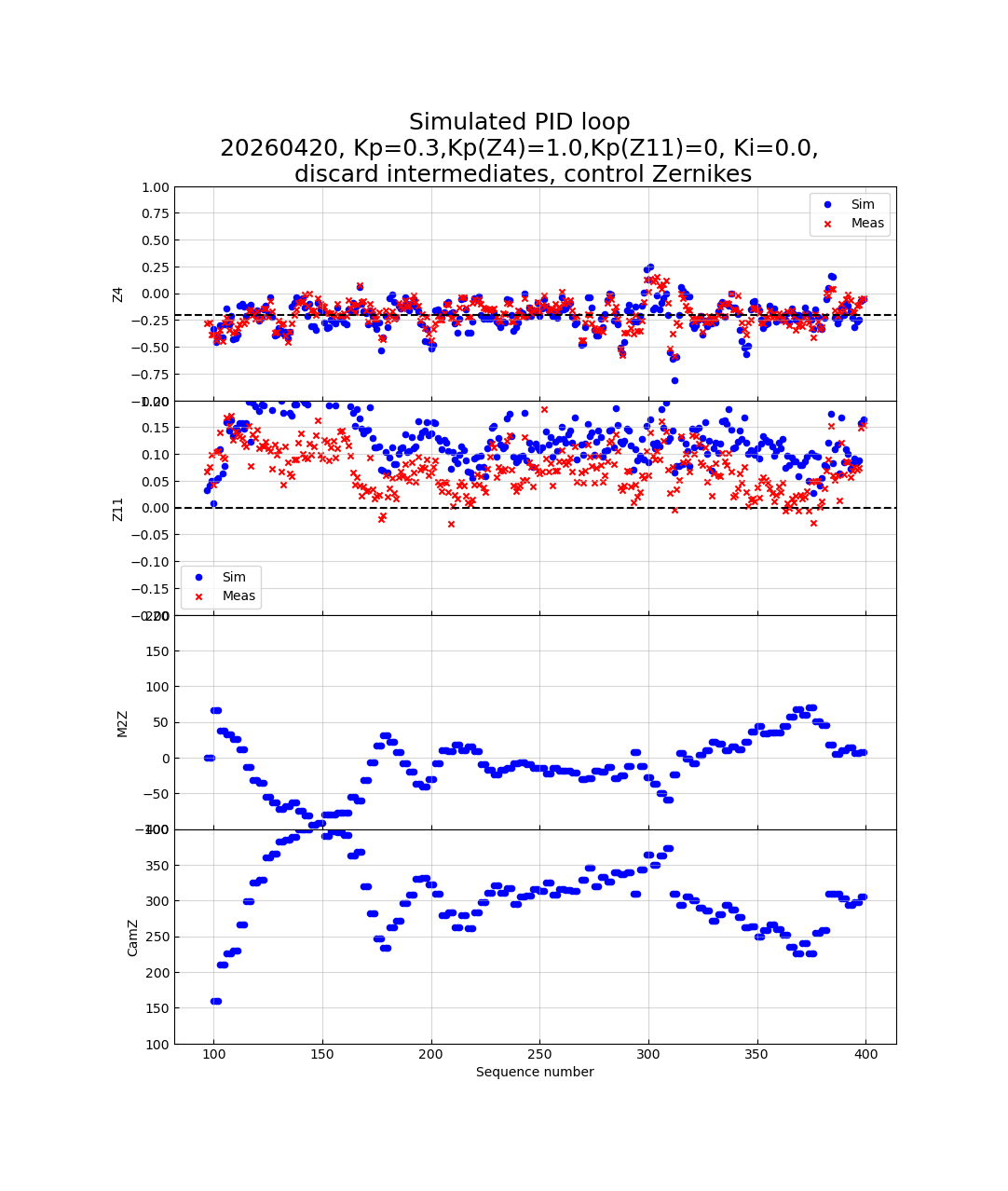
• Setting Kp(Z11) = 0 reduces but does not eliminate the CamZ and M2Z oscillations, indicating residual coupling through other Vmodes.

Fig. 31 shows an example run with Kp(Z4) = 1.0 and all other Zernikes at Kp = 0.3. Fig. 32 and Fig. 33 compare the Z4/Z11 cross-coupling with and without zeroing the Z11 gain.

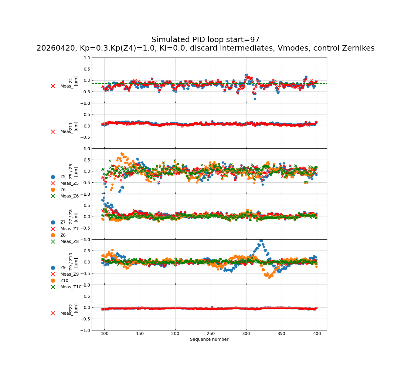
Fig. 31 Zernike-space control, night 20260420. Kp=0.3 for all Zernikes, Kp(Z4)=1.0. Simulated Zernikes (circles) and measured Zernikes (crosses) are shown.

Fig. 32 Kp(Z4)=1.0, all other Kp=0.3. Z4 is well controlled; M2Z and CamZ show large swings.

Fig. 33 Kp(Z4)=1.0, Kp(Z11)=0.0. Z11 is no longer driven, but M2Z and CamZ swings persist.

Plotting Options

There are three plotting options built in to the simulation class, shown in Fig. 34 through Fig. 36.

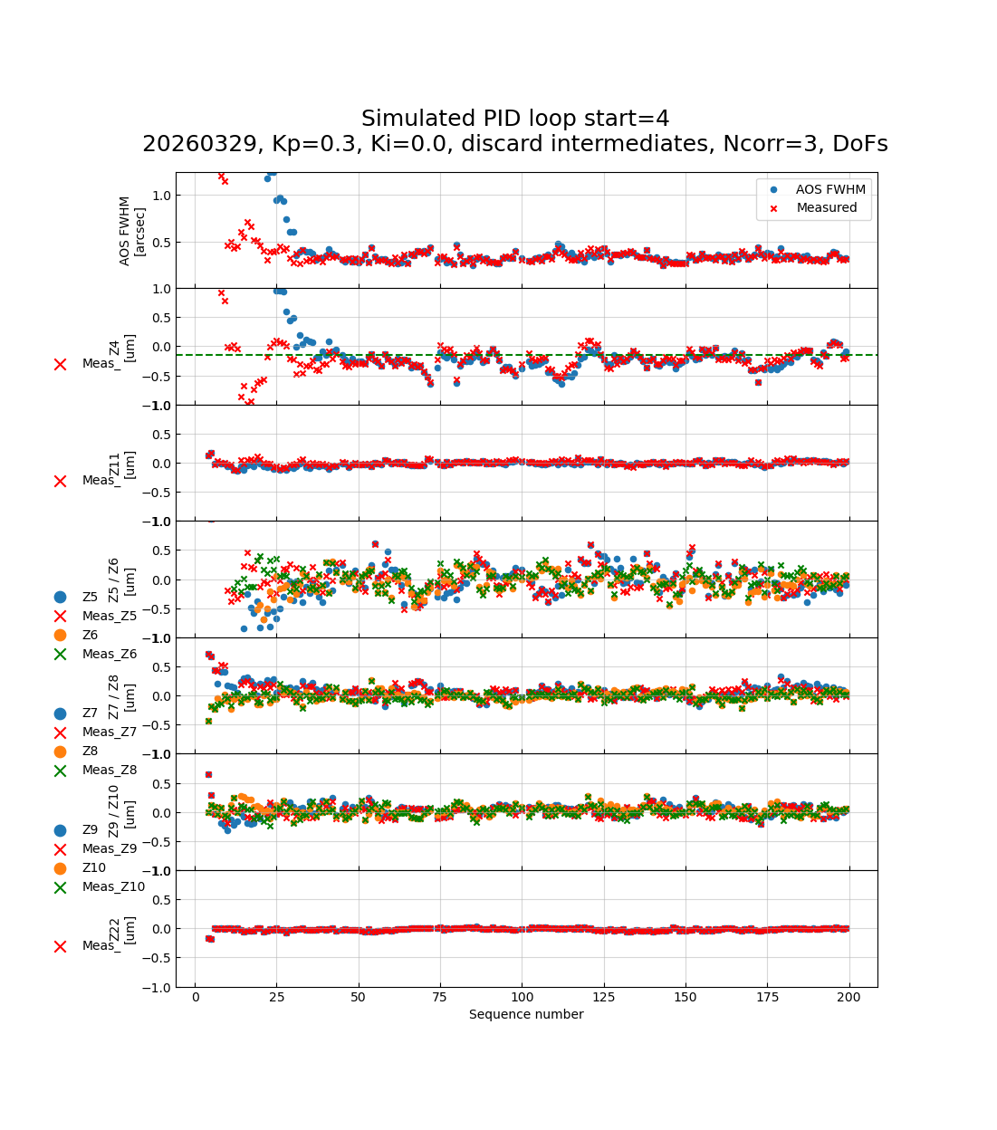
Fig. 34 The simplest plotting option (plotPID) shows the AOS FWHM and the six most important Zernike groups vs. sequence number.

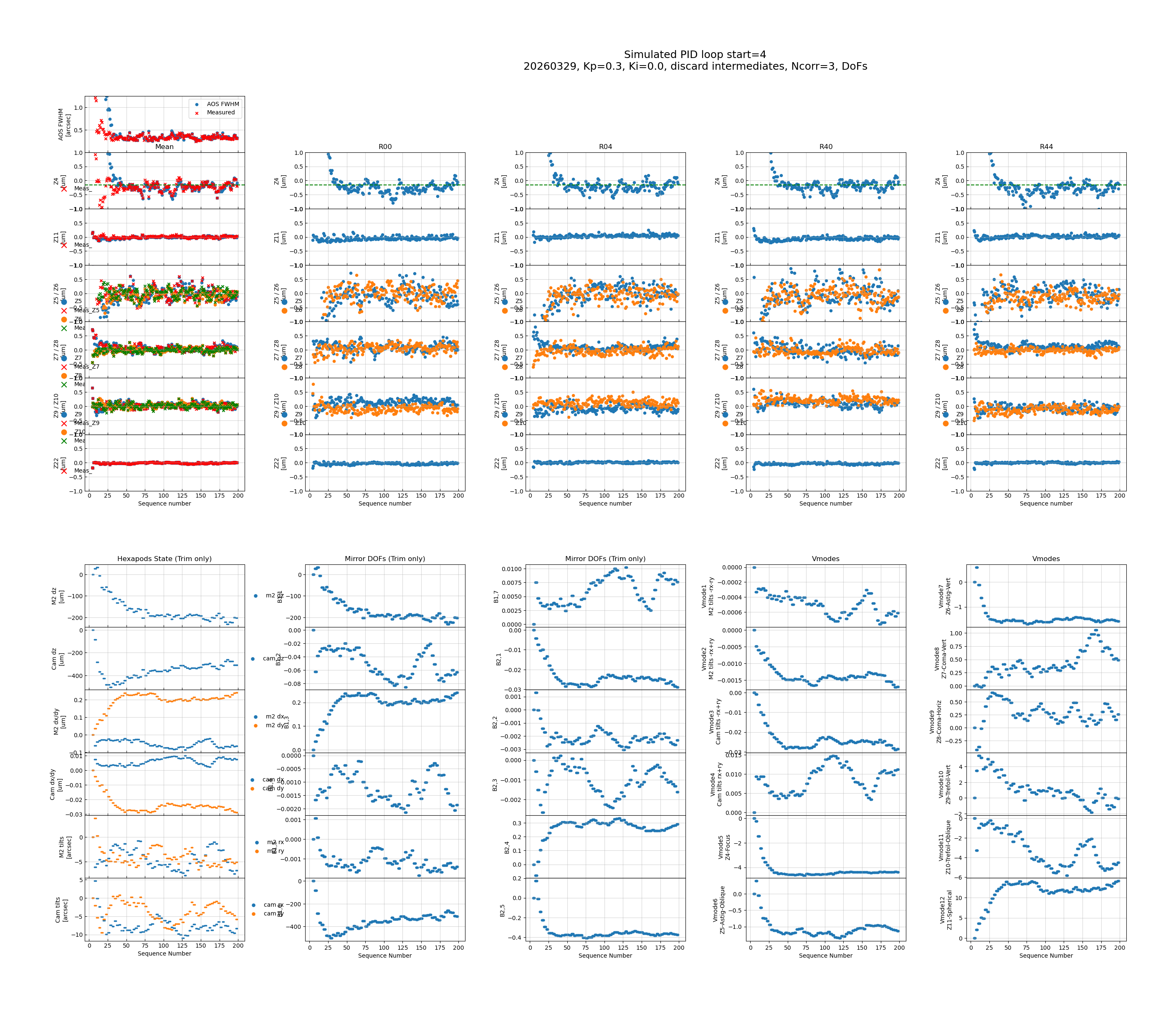
Fig. 35 bigPlotPID1 adds the Zernikes at all four corner detectors (top panel) and all DoF trims and Vmodes (bottom panel).

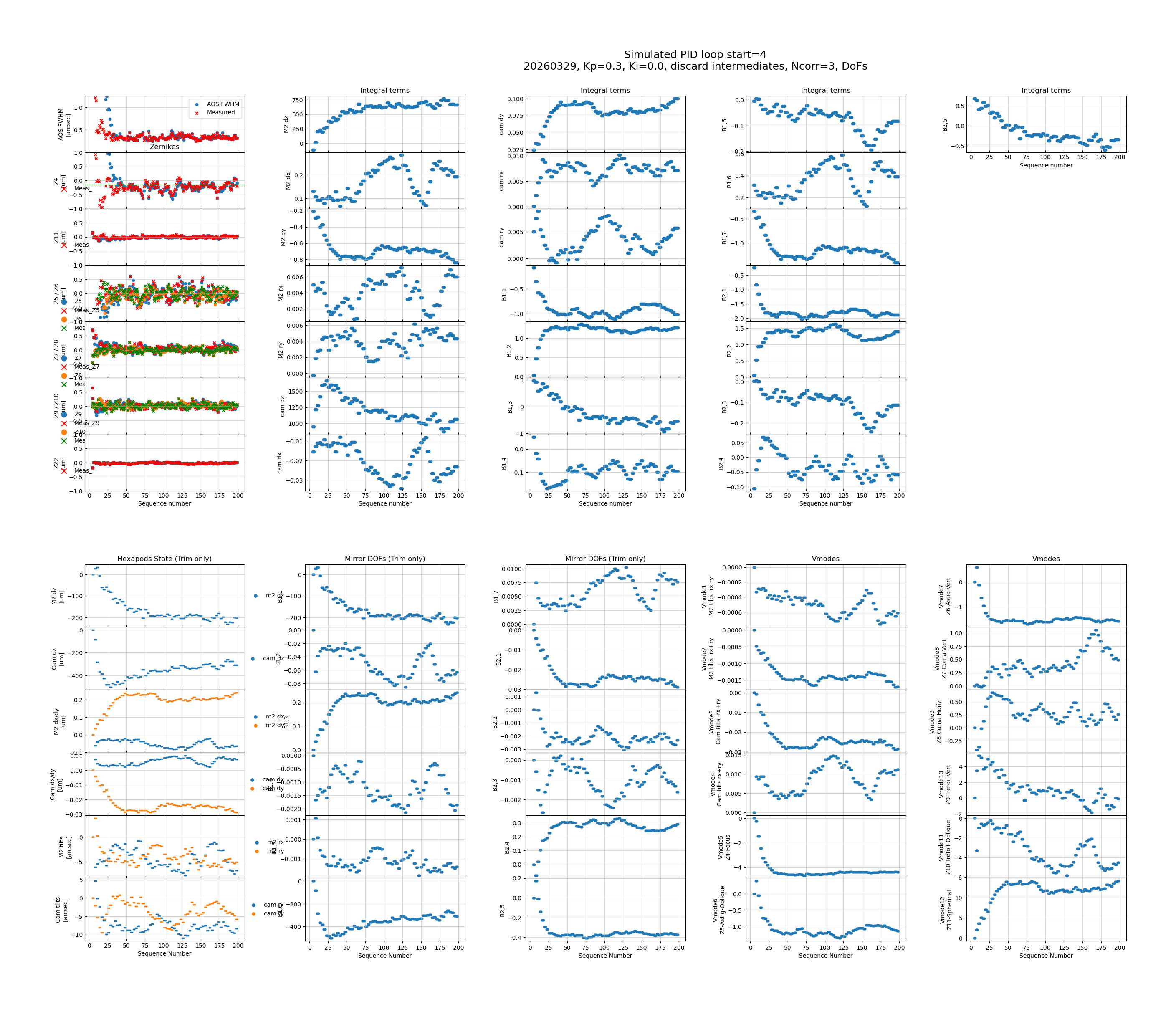
Fig. 36 bigPlotPID2 replaces the per-corner Zernike columns with plots of the integral terms for all active DoFs.

Adding the Kalman Filter

Methodology

The Zernike measurements from the corner detectors are noisy (typical RMS ~0.05 µm per mode), which limits the achievable PID gain. A Kalman filter can be inserted between the applyTrim step and the getTweak step to produce an improved state estimate before the correction is calculated. The overall design is shown in Fig. 37.

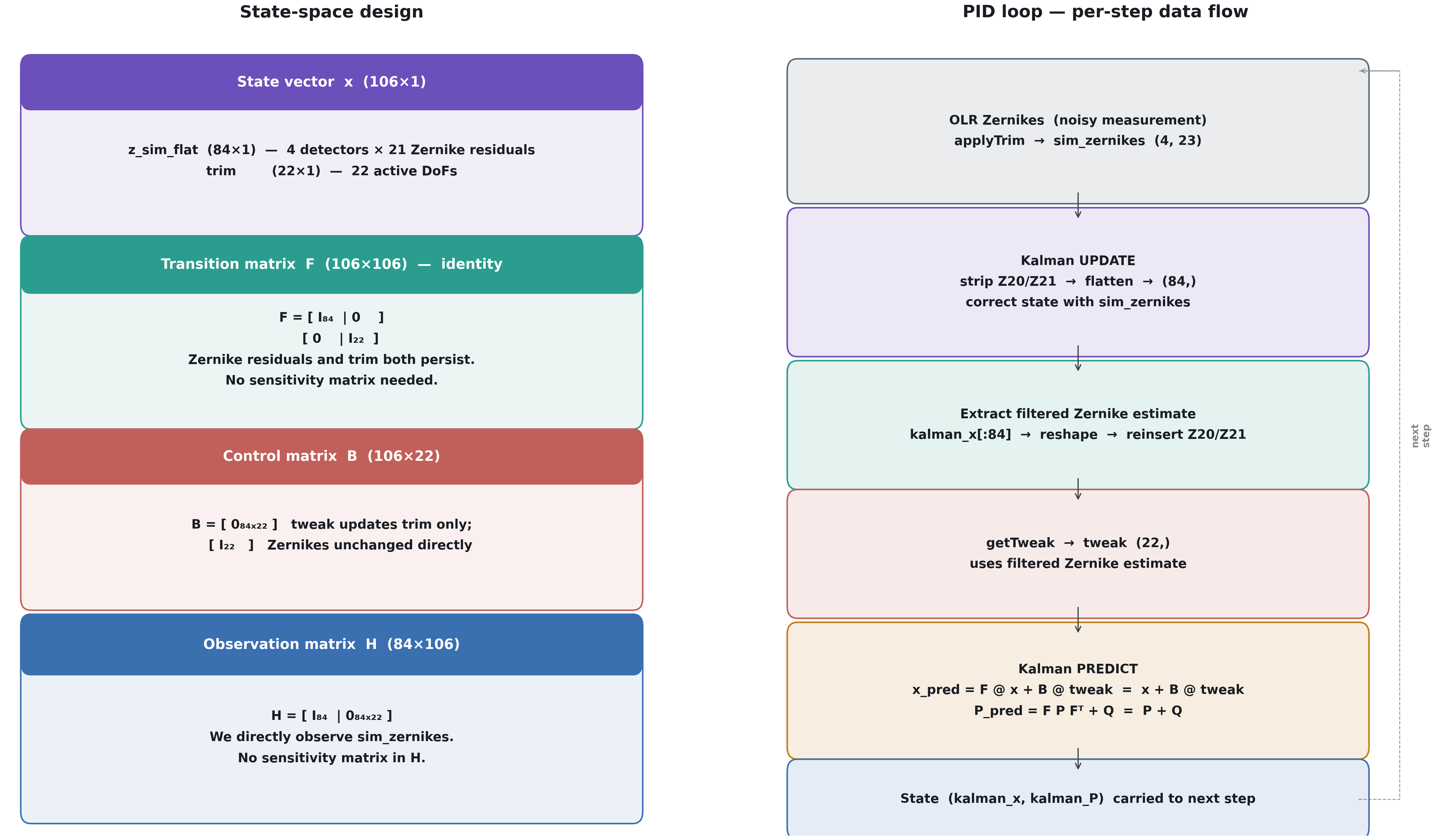
Fig. 37 Left: the four matrices that define the Kalman filter in state space. Right: the per-step data flow showing where the update and predict phases sit within the PID loop.

The filter operates on a 106-element state vector composed of the 84 active OFC Zernike values (4 detectors × 21 modes, excluding Z20/Z21) and the 22 active DoF trim values:

\[\begin{split}\mathbf{x} = \begin{pmatrix} \mathbf{z}_\mathrm{flat} \\ \mathbf{t} \end{pmatrix}\end{split}\]

The state transition matrix \(F\) at present is simply the identity matrix, so the trim and zernike values persist between visits. This formulation of the Kalman filter needs discussion.

\[F = \begin{pmatrix} I_{106} \end{pmatrix}\]

A control-input matrix \(B = [0_{84 \times 22};\; I_{22}]^T\) propagates the applied tweak into the trim state each visit. The observation matrix \(H = [I_{84}\;|\;0_{84 \times 22}]\) selects only the Zernike block, since we observe Zernikes but not the trim directly.

The update and predict steps follow the standard Kalman equations. The filter is enabled with use_kalman=True and is configured by three covariance parameters:

• kalman_r_sigma — standard deviation of Zernike measurement noise (default 0.05 µm); sets \(R = \sigma_R^2 I_{84}\). There is also the option to enter the kalman_r matrix directly.

• kalman_q_z_sigma — process noise on the Zernike block (default 1×10⁻⁴ µm; Zernikes evolve slowly between visits).

• kalman_q_trim_sigma — process noise on the trim block (default 1×10⁻⁶ µm; trim is updated deterministically via \(B\)).

When use_kalman=False (the default) the simulation is identical to the non-Kalman case.

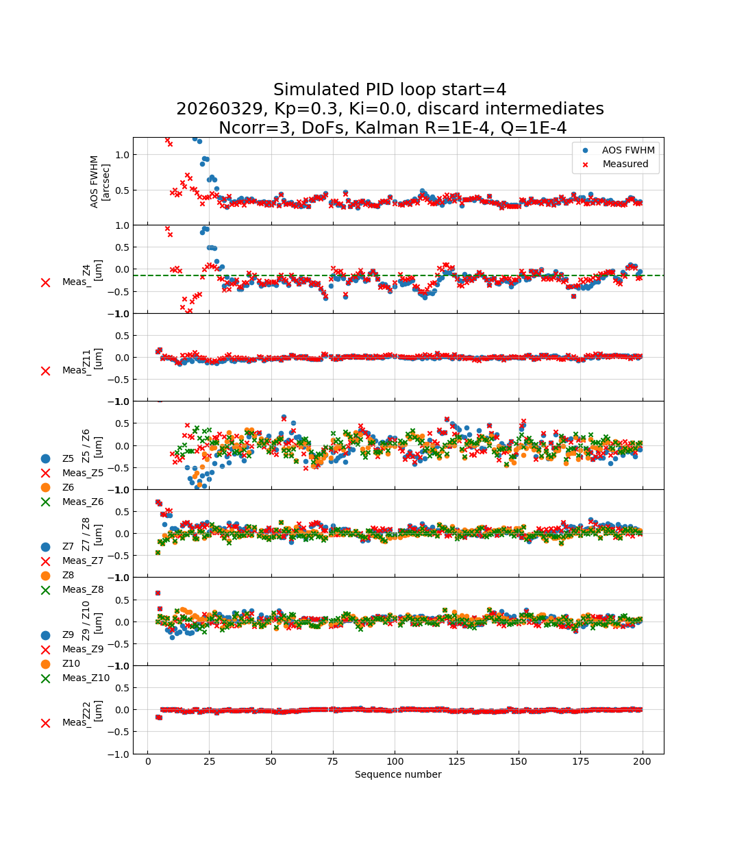
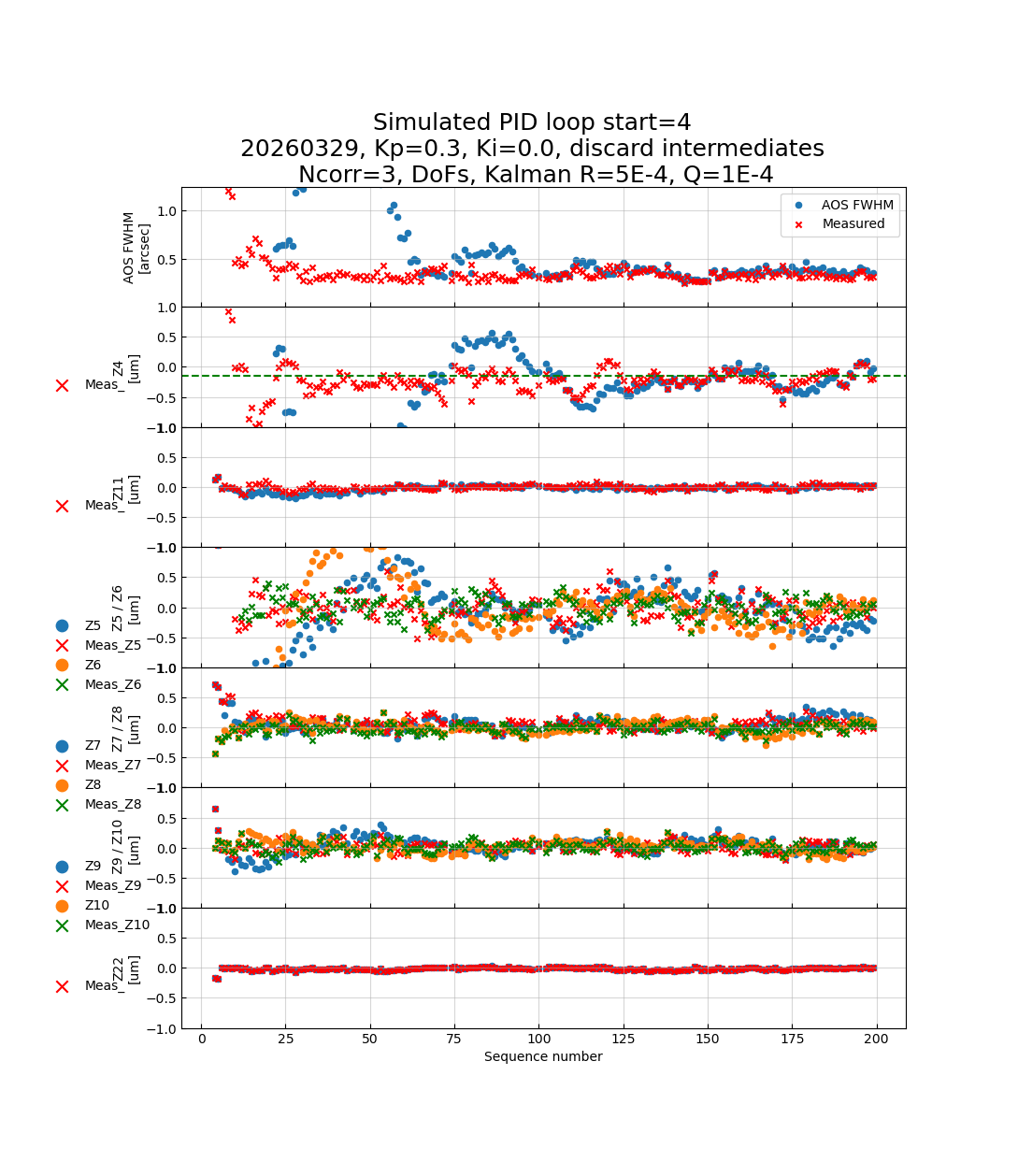
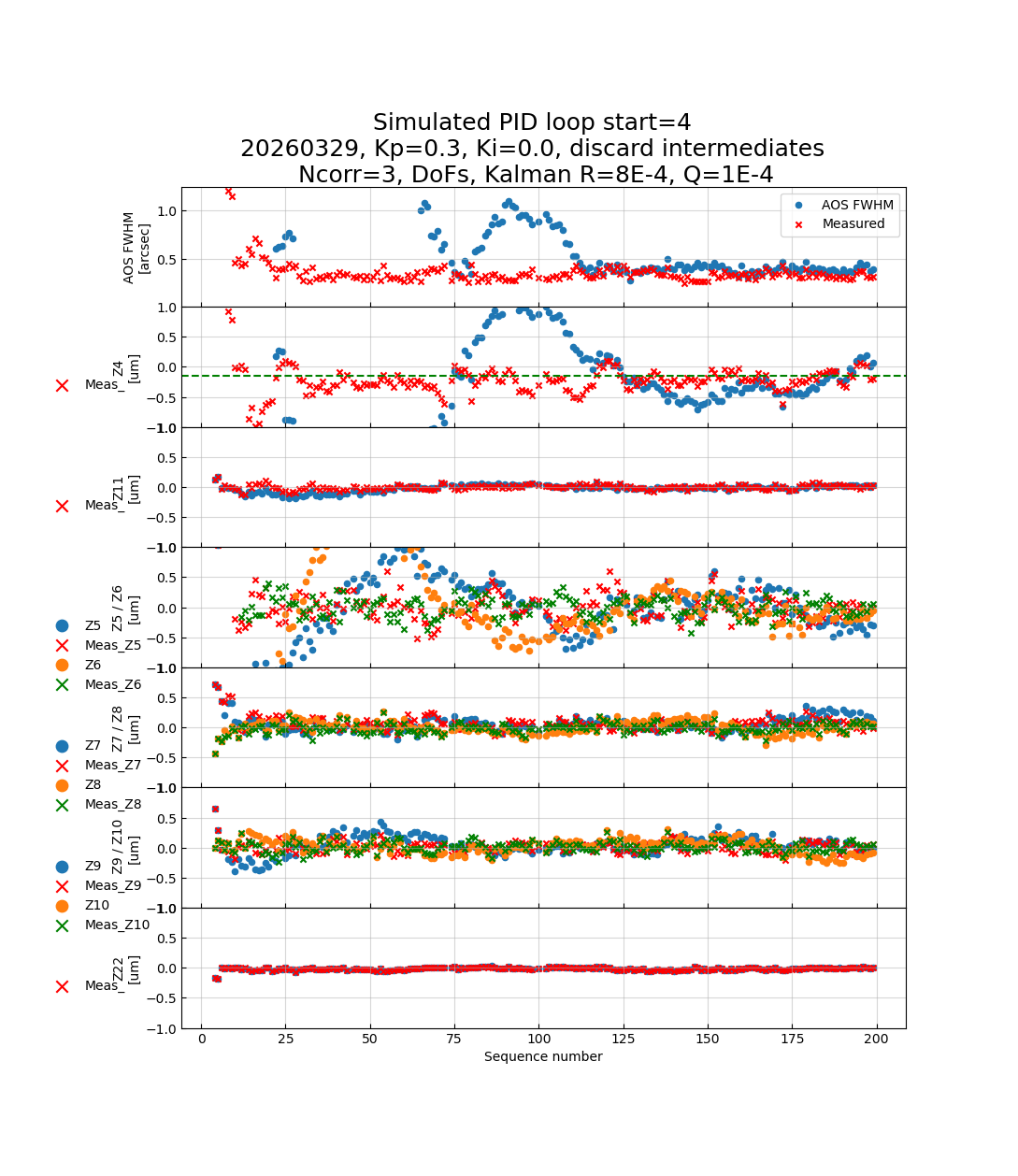
Results

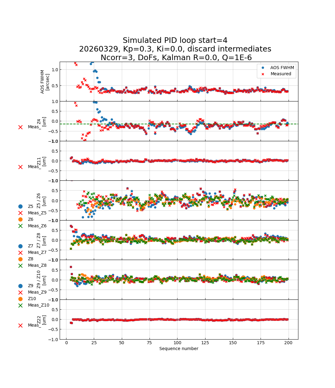
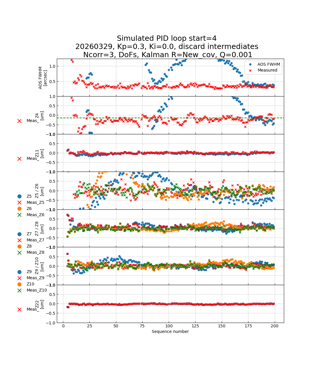
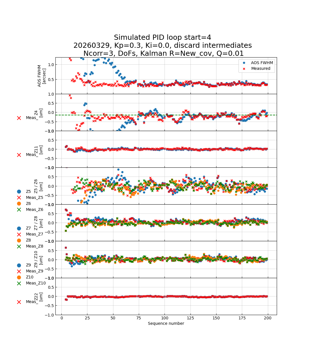
The Kalman filtering methodology is new, but there are some initial results. Fig. 38 through Fig. 41 show what happens when the R matrix of measurement errors is a multiple of the identity with a given sigma. When the sigma is zero, the measurements are assumed perfect and no Kalman filtering is done. As the sigma increases, the loop converges more slowly until it fails to converge at all.

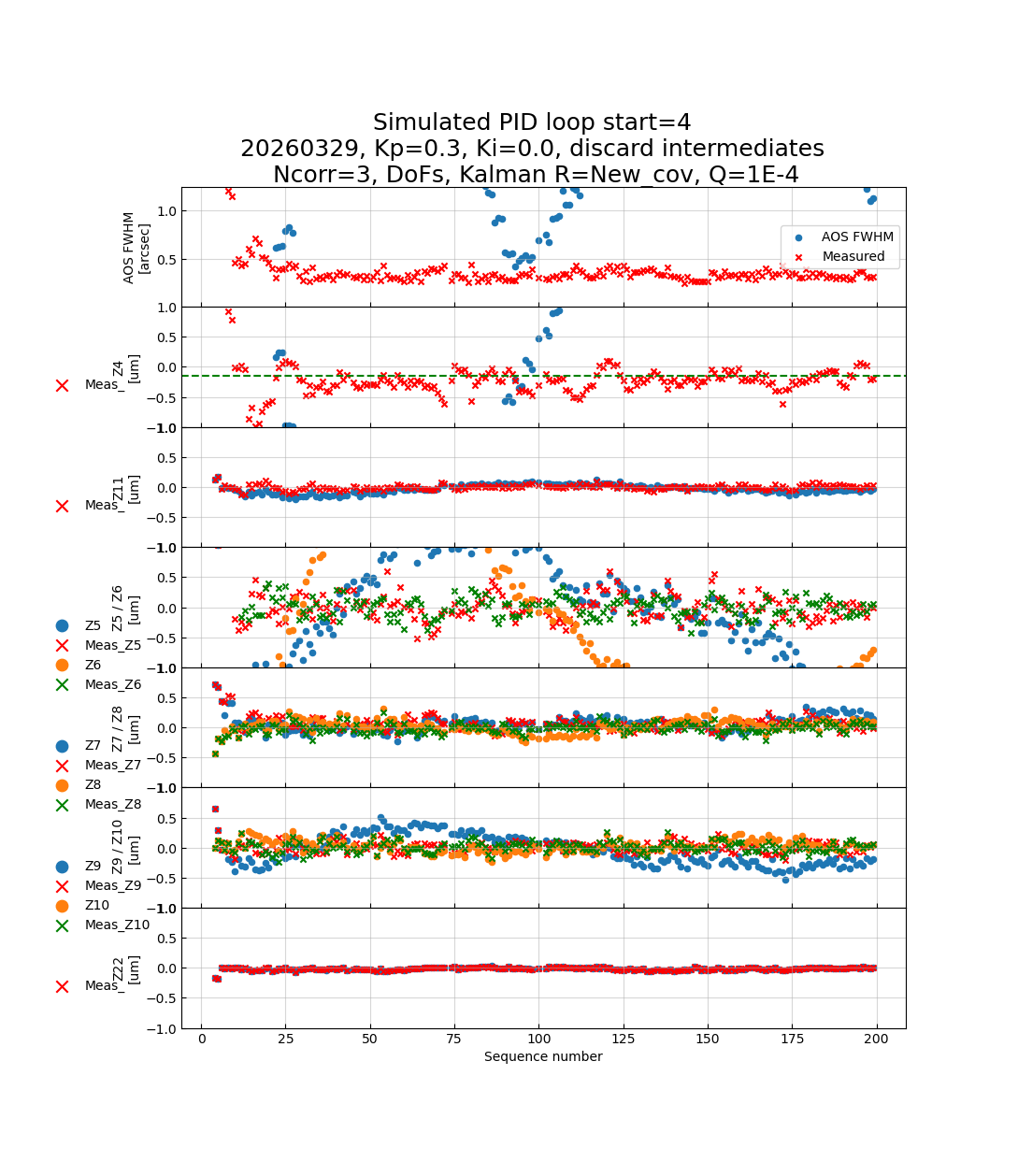
Fig. 42 through Fig. 45 use the Zernike covariance matrix originally calculated by Bo Xin. The R matrix and the Q matrix together determine how the Kalman filtering takes place: when \(R \ll Q\) the measurements take precedence and little filtering is done; when \(Q \ll R\) the model dominates over the measurements. In order to use the calculated covariance matrix, the Q sigmas needed to be increased substantially for the loop to converge. Much more study is needed to determine:

• Whether the Kalman filter is coded correctly.

• Whether it will be useful in our control loops.

• What the proper R and Q matrices should be.

As of this writing, no benefit to the Kalman filtering is seen, but hopefully with code or parameter improvements a benefit will be demonstrated.

Fig. 38 R-matrix sigma = 0. The Kalman filter has no impact, as expected.	Fig. 39 R-matrix sigma = 1×10⁻⁴. Similar to R_sigma = 0.0.
Fig. 40 R-matrix sigma = 5×10⁻⁴. Control converges more slowly.	Fig. 41 R-matrix sigma = 8×10⁻⁴. Control converges more slowly still.

Fig. 42 R=calculated covs both Q sigmas = 1E-4.	Fig. 43 R=calculated covs both Q sigmas = 1E-3.
Fig. 44 R=calculated covs both Q sigmas = 0.01.	Fig. 45 R=calculated covs both Q sigmas = 0.1.

Conclusions and Future Work

The open-loop reproduction PID simulator has proved to be a useful tool for understanding and optimising the MTAOS control loop without consuming on-sky time. Key findings from the first round of simulations are:

• Correction lag causes oscillations. Keeping intermediate updates with a large correction lag leads to loop oscillations, particularly for higher gains. Discarding intermediate updates eliminates this instability at the cost of slower convergence. However, with a correction lag of two — which we expect to be routinely achievable in the future — the oscillation problem is much reduced, and it may be possible to return to keeping intermediate updates for faster response.

• The Smith predictor/corrector reduces oscillations. Adding the Smith correction term substantially reduces Zernike scatter in the keep-intermediates regime and allows higher gains to be used stably. However, it appears less useful when the lag is reduced from three visits to two.

• DoF and Vmode control are equivalent for the same gain values. Internally the OFC always projects corrections onto the Vmode basis, so the two control modes produce identical Zernike residuals.

• Per-mode gain tuning is effective. Reducing the gain on individual Vmodes (particularly Vmode 10/Z11-spherical) can reduce unwanted cross-coupling at the expense of slower correction of that mode.

• Integral control on individual Vmodes can reduce low-frequency drift but must be tuned carefully to avoid instability.

• Zernike-space control offers fine-grained per-coefficient gain control but its interaction with the OFC’s internal DoF basis needs further investigation.

Planned future work:

• Validate and tune the Kalman filter to determine whether it allows higher stable gains and smaller Zernike residuals.

• Investigate the bending-mode saturation hypothesis to explain nights where the simulation does not recover the measured Zernikes.

• Explore the full parameter space of Kp, Ki, and max_integral.

• Test the Zernike-space control mode more systematically.

• Consider adding simulated measurement noise to the OLR stream to enable quantitative evaluation of the Kalman filter.